Google’s DeepMind is one of the world’s foremost AI research teams. They’re most famous for creating the AlphaGo player that beat South Korean Go champion Lee Sedol in 2016.
The key technology used to create the Go playing AI was Deep Reinforcement Learning.
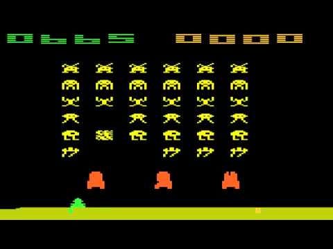
Space Invaders!
Let’s go back 4 years, to when DeepMind first built an AI which could play Atari games from the 70s. Games like Breakout, Pong and Space Invaders. It was this research that led to AlphaGo, and to DeepMind being acquired by Google.
Today we’re going to take that original research paper and break it down paragraph-by-paragraph. This will make it more approachable for people who only just now started learning about Reinforcement Learning. And for those who don’t use English as their first language (which makes it VERY difficult to read such papers).
Here’s the original paper if you want to try reading it:
https://arxiv.org/pdf/1312.5602v1.pdf
Some quick notes (in case you don’t make it to the bottom of this 20-minute article)
The explanations here are by two people:
- Me, a self driving cars engineer
- Qiang Lu, a PhD candidate and researcher at the University of Denver
We hope that our work will save you a lot of time and effort if you were to study this on your own.
And if you’re more comfortable reading Chinese, here is an *unofficial* translation of this essay.
- We love your claps, but love your comments even more. Unload whatever is on your mind — feelings, suggestions, corrections, or criticism — into the comment box!
If you are interested in joining a discussion (invite-only) about this and other high-quality research papers, you should visit DenseLayers.
Let’s get started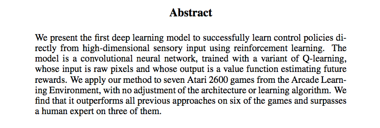
We want to make a robot learn how to play an Atari game by itself, using Reinforcement Learning.
The robot in our case is a convolutional neural network.
This is almost real end-to-end deep learning, because our robot gets inputs in the same way as a human player — it directly sees the image on the screen and the reward/change in points after each move, and that is all the information it needs to make a decision.
And what does the robot output? Well, ideally we want the robot to pick the action which it thinks promises the most reward in future. But instead of directly choosing the action, here we let it assign “values” to each of the 18 possible joystick actions. So put simply, the value V for any action A represents the robot’s expectation of the future reward it will get if it performs that action A.
So in essence, this neural network is a value function. It takes as input the screen state and change in reward, and it outputs the different values associated with each possible action. So that you can pick the action with the highest value, or pick any other action based on how you program the overall player.
Say you have the game screen, and you want to tell a neural network what’s on the screen. One way would be to directly feed the image into the neural network; we don’t process the inputs in any other way. The other would be to create a summary of what’s happening on the screen in a numerical format, and then feed that into the neural network. The former is being referred to here as “high dimensional sensory inputs” and the latter is “hand crafted feature representations.”
Read abstract explanation. Then this paragraph is self-explanatory.
Deep Learning methods don’t work easily with reinforcement learning like they do in supervised/unsupervised learning. Most DL applications have involved huge training datasets with accurate samples and labels. Or in unsupervised learning, the target cost function is still quite convenient to work with.
But in RL, there’s a catch — as you know, RL involves rewards which could be delayed many time steps into the future (for example it takes several moves to knock the opponent’s queen in chess, and each of those moves doesn’t return the same immediate reward as the final move, EVEN IF one of those moves might be more important than the final move).
The rewards could also be noisy — for instance, sometimes the points for a particular move are slightly random and not easily predictable!
Moreover, in DL usually the input samples are assumed to be unrelated to each other. For example in an image recognition network, the training data will have huge numbers of randomly organized and unrelated images. But while learning how to play a game, usually the strategy of moves doesn’t just depend on the current state of the screen but also some previous states and moves. It’s not simple to assume no correlation.
Now, wait a second. Why is it important for our training data samples to not be correlated to each other? Say you had 5 samples of animal images, and you wanted to learn to classify them into “cat” and “not cat”. If one of those images is of a cat, does it affect the likelihood of another image also being a cat? No. But in a video game, one frame of the screen is definitely related to the next frame. And to the next frame. And so on. If it takes 10 frames for a laser beam to destroy your spaceship, I’m pretty sure the 9th frame is a pretty good indication that the 10th frame is going to be painful. You don’t want to treat the two frames just a few milliseconds apart as totally separate experiences while learning, because they obviously carry valuable information about each other. They’re part of the same experience — that of a laser beam striking your spaceship.
Even the training data itself keeps changing in nature as the robot learns new strategies, making it harder to train on. What does that mean? For example, say you’re a noob chess player. You start out with some noob strategies when you play your first chess game, i.e keep moving forward, kill the pawn on the first chance you get etc. So as you keep learning those behaviors and feel happy taking pawns, those moves act like your current training set.
Now one day you try out a different strategy — sacrificing one of your own bishops to save your queen and take the other’s rook. Bam you realize this is so amazing. You’ve added this new trick to your training set, which you would never have learned if you had kept just practicing your previous noob strategy.
This is what it means to have a non-stationary data distribution, which doesn’t really happen in supervised/unsupervised learning.
So given these challenges, how do you even train the neural network in such a situation?
In this paper we show how we overcame the above mentioned problems AND we directly used raw video/image data. Which means we’re awesome.
One specific trick that is worth mentioning: “Experience Replay”. This solves the challenge of ‘data correlation’ and ‘non-stationary data distributions’ (see previous paragraph to understand what these mean).
We record all our experiences — again using the chess analogy, each experience looks like [current board status, move I tried, reward I got, new board status] — into a memory. Then while training, we pick up randomly distributed batches of experiences which aren’t related to each other. In each batch, different experiences could be associated with different strategies as well — because all the previous experiences and strategies are now jumbled together! Make sense?
This makes the training data samples more random and un-correlated, and it also makes it feel more stationary to the neural network because every new batch is already full of random strategy experiences.
Much of it is self-explanatory. The key here is that the exact same neural network architecture and hyperparameters (learning rate, etc) were used for each different game. It’s not like we used a bigger network for space invaders and a smaller network for ping-pong. We did train the networks from scratch for each new game, but the network design itself was the same. That’s pretty awesome right?
First couple sentences are self-explanatory. By saying that ‘E’ is stochastic, it means that the environment is not always predictable (which is true in games right? anything could happen at any time).
It also repeats that the neural network does NOT get any information about the internal state of the game. For example, we don’t tell it things like “there’s a monster at this position who is firing at you and moving in this direction, your spaceship is present here and moving there, etc”. We simply give it the image and let the convolutional network figure out by itself where the monster is, and where the player is, and who is shooting where etc. This is to make the robot train in a more human-like way.
Perceptual Aliasing: Meaning that two different states/places can be perceived as the same. For example, in a building, it is nearly impossible to determine a location solely with the visual information, because all the corridors may look the same.
Perceptual aliasing is a problem. In Atari games the state of the game doesn’t change so much in every millisecond, nor is a human being capable of making decisions in every millisecond. So when we take video input at 60 frames per second, and treat each frame as a separate state, then most of the states in our training data will look exactly the same! It’s better to keep a longer horizon for what a “state” looks like, which has, say, at least 4 to 5 frames (say). Multiple consecutive frames also contain valuable information about each other — for example, a still photograph of two cars a foot away from each other is very ambiguous — is one car about to crash into the other? Or are they about to move away from each other after coming this close? You don’t know. But if you take 4 frames from the video and see them one after the other, now you know how the cars are moving and can guess if they’re going to crash or not. We call this a sequence of consecutive frames, and use one sequence as a state.
Moreover, when a human moves the joystick it usually stays in the same position for several milliseconds, so that is incorporated into this state. The same action is continued in each of the frames. Each sequence (which includes several frames and the same action between them) is an individual state, and this state still fulfils a Markov Decision Process (MDP).
If you’ve read up on RL, you’d know what MDPs are and what they mean! MDPs are the core assumption in RL.
Now, to understand this part you should really do some background study into Reinforcement Learning and Q-Learning first. It’s very important. You should understand what the Bellman equation does, what discounted future rewards are etc. But let me try to give a really simple overview of Q-learning.
Remember what I said about “value function” earlier? Scroll up to the Abstract and read it.
Now, let’s say you had a table which had a row for ALL the possible states (s) of the game, and the columns represented all the possible joystick moves (a). Each cell in the row represents the maximum total future value possible if you take that particular action and play your best fro then on. This means you now have a “cheat sheet” of what to expect from any action at any state! The values of these cells is called the Q-star value. (Q*(s,a)). For any state s, if you take action a, the maximum total future value is Q*(s,a) as seen in that table.
In the last line, pi is ‘policy’. Policy is simply the strategy about what action to pick when you are in a particular state.
Now, if you think about it, say you are in state S1. You see the Q* value for all possible actions in the table (explained in para3), and choose A1 because its Q value is the highest. You get an immediate reward R1, and the game moves into a different state S2. For S2, the max future reward will be if it takes (say) action A2 in the table.
Now, the initial Q value Q*(S1,A1) is the max value you could get if you played optimally from then on, right? This means, that Q*(S1, A1) should be equal to the sum of the reward R1 AND the max future value of the next state Q*(S2,A2)! Does this make sense? But hey we want to reduce the influence of the next state, so we multiply it by a number gamma which is between 0 and 1. This is called discounting Q*(S2,A2).
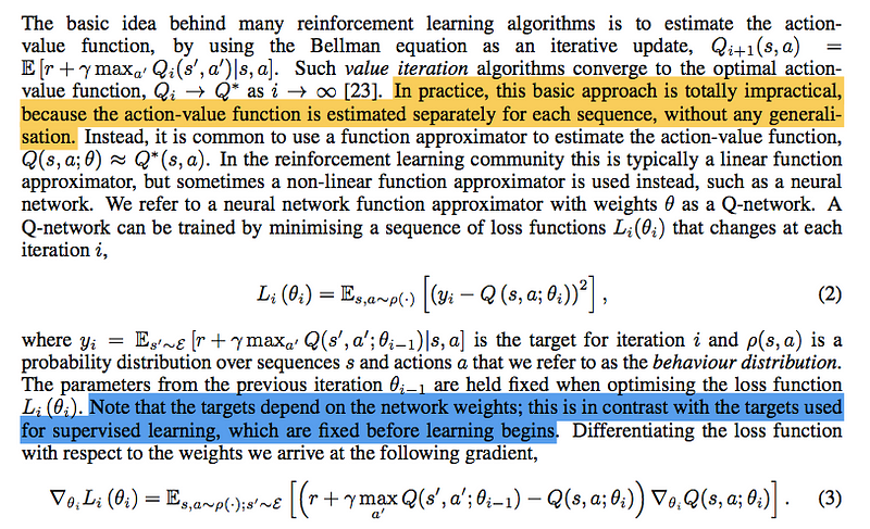
I’ll admit, this one won’t be easy to grasp just by reading my explanation. Put some time here.
Therefore Q*(S1,A1) = R1 + [gamma x Q*(S2,A2)]
Look at the previous equation again. We’re assuming that for any state, and for any future action, we *know* the optimal value function already, and can use it to pick the best action at the current state (because by iterating over all the possible Q values we can literally look ahead into the future). But of course, such a Q-function doesn’t really exist in the real world! The best we can do is *approximate* the Q function by another function, and update that approx function little by little by testing it in the real world again and again. This approx function can be a simple linear polynomial, but we can even use non-linear functions. So we choose to use a neural network to be our “approximate Q function.”
Now you know why we’re reading this paper in the first place — DeepMind uses a neural network to approximate a Q function, and then they let the computer play ATARI games using the network to help predict the best moves. With time, as the computer gets a better and better idea of how the rewards work, it can tweak its neural network (by adjusting the weights), so that it becomes a better and better approximation of that “real” Q function! And by the time that approximation is good enough, voila we realize it can actually make better predictions than humans.
Now, leaving aside some of the mathematical mumbo jumbo above (it’s hard for me too!). Know that Q-learning is a *model-free* approach. When you say “model-free” RL, it means that your agent doesn’t need to explicitly learn the rules or physics of the game. In model-based RL, those rules and physics are defined in terms of a ‘Transition Matrix’ which calculates the next state given a current state and action, and a ‘Reward Function’ which computes the reward given a current state and action. In our case these two things are too complex to calculate, and if you think about it, we don’t really need them! In our “model free” approach, we simply care about learning the Q value function with hit and trial, because we assume that a good Q function will inherently have to follow the rules and physics of the game.
Our approach is also *off-policy*, and not *on-policy*. The difference here is more subtle because in this paper they’ve followed a hybrid of sorts. Assume you’re at state s and have several actions to choose from. We have an approximate Q value function, so we calculate what will be the Q value for each of those actions. Now, while choosing the action, you have two options. The “common sense” option is to simply choose the action that has the highest Q value right? Yes, and this is what’s called a “greedy” strategy. You always pick the action which seems best to you *right now, given your current understanding of the game* — in other words, given your current approximate of the Q function — which means, given your current strategy. But there lies the problem — when you start out, you don’t really have a good Q function approximator right? And even if you have a somewhat good strategy, you still want your AI to check out other possible strategies and see where they lead. This is why a “greedy” strategy isn’t always the best when you’re learning. While learning, you don’t want to just keep trying what you believe will work — you want to try other things which seem less likely, just so you can get experience. And that’s the difference between on-policy (greedy) and off-policy (not greedy).
Why did I say we use a hybrid of sorts? Because we vary the approach based on how much we’ve learned. We vary the probability with which the agent will pick the greedy action. How do we vary that? We pick greedy actions with a probability of (1-e), where e is a variable that represents how random the choice is. So e=1 means the choice is completely random, and e=0 means that we always pick the greedy action. Makes sense? At first, when the network just begins learning, we pick e to be very close to 1, because we want the AI to explore as many strategies as possible. As time goes by and the AI learns more and more, we reduce the value of e towards 0 so that the AI stays on a particular strategy.
Qiang: The backgammon game is the most popular game for scientists to test their various artificial intelligence and machine learning algorithms. Reference [24] used a model-free algorithm to achieve a superhuman level of play. Model-free means there is not a explicit equation between the algorithm’s input (screen images) and output (best play strategy found).
Q-learning, where ‘Q’ stands for ‘quality’, uses a Q function which represents the maximum discounted future reward when we perform a certain action in a certain state. Then the optimal policy (play strategy) is continually found from that point on. The difference in reference [24] is that they are using approximation for the q-value using a multi-layer perceptron (MLP). In their MLP, one hidden layer exists between the output layer and the input layer.
Qiang: The unsuccessful following applications of similar methods on other games made people don’t believe TD-gammon approach. They owe the success of TD-gammon on backgammon to the stochasticity of dice rolls.
Go a few paragraphs back, where we saw what kinds of functions can be used to approximate our theoretically perfect Q-function. Apparently, linear functions are better suited to the task than non-linear functions like neural networks, because they make the network easier to ‘converge’ (i.e the weights adjust in such a way that the networks makes more accurate, instead of becoming more random).
Qiang: In recent time, combining deep learning with reinforcement becomes research interest again. Environment, value function, and policy have been estimated by deep learning algorithms. In the meantime, the divergence has been partially solved by gradient temporal-difference methods. However, as mentioned in the paper, these methods can only works with nonlinear function approximator not directly with nonlinear function.
Qiang: NFQ is the most similar prior work to the approach in this paper. Main idea of NFQ is using RPROP (resilient backpropagation) to update the parameters of the Q-network to optimise the sequence of loss functions in Equation 2. The disadvantages of NFQ is that it introduced computational cost which is proportional to the size of data set because of batch update.
This paper uses stochastic gradient updates which is computationally efficient. The NFQ applied on simple tasks but not on the visual input, this paper’s algorithm learns end-to-end. Another paper about Q-learning also used low-dimensional state instead of raw visual inputs which is the advantage of this paper.
Qiang: This paragraph introduced several applications of the Atari 2600 emulator. The first paper that used the Atari 2600 emulator as a reinforcement learning platform applied standard reinforcement learning algorithms with linear function approximation and generic visual features. Larger number of features, and project features to lower-dimensional space improved the results. And the HyperNEAT evolutionary architecture evolved respectively a neural network for each game. And the neural network represents the play strategy, which were able to be trained and exploit some design flaws in some games.
But as mentioned in the paper, this paper’s algorithm learns the strategy for seven Atari 2600 games without adjustment of the architecture. This is the big advantage of the algorithm in this paper.
Self explanatory?
TD Gammon was an on-policy approach, and it directly used the experiences (s1, a1, r1, s2) to train the network (without experience replay etc).
Now we come to the specific improvements made over TD Gammon. The first of these is experience replay, which has already been talked about previously. The ‘phi’ function does image preprocessing etc, so the state of the game is stored as the final preprocessed form (more on this in the next section)
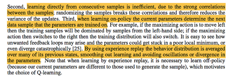
These are the concrete advantages of using experience replay (this paragraph continues on the next page). Firstly, just like in regular deep learning, where each data sample can be reused multiple times to update weights, we can use the same experience multiple times while training. This is more efficient use of data.
Second and third are very related. Because each state is very closely related to the next state (as it is while playing a video game), then training the weights with each consecutive state will lead to the program only following one single way of playing the game. You predict a move based on Q function, you make that move, and update the weights so that the next time you will again likely move left. But by breaking this pattern and drawing randomly from past experiences, you can avoid these feedback loops.
Now, it’s good to draw random samples from experience replay, but sometimes in a game there are important transitions that you would like the agent to learn about. This is a limitation of the current approach in this paper. A suggestion given is to pick important transitions with a greater probability while using experience replay. Or something like that.
(Beyond this point, everything is based on the theory covered in the previous sections so a lot of it is just technical details)
Most of this is self-explanatory. The state S is preprocessed to include 4 consecutive frames, all preprocessed into grayscale and resized and cropped to 84×84 squares. I think this is because given that the game runs at over 24 frames per second, and humans can’t react so fast as to make a move in each single frame, it makes sense to consider 4 consecutive frames as being in the same state.
While making the network architecture, you can either make it a Q function which takes both S1 and A1 and outputs Q-value for this combination. But this means that you’d have to run this network for each of the 18 possible joystick actions at each step, and compare the output of all 18 runs. Instead, you can simply have an architecture where you use S1 as input and have 18 outputs each corresponding to the Q-value for a given joystick action. It’s much more efficient to compare the Q-values in this way!
Self explanatory :)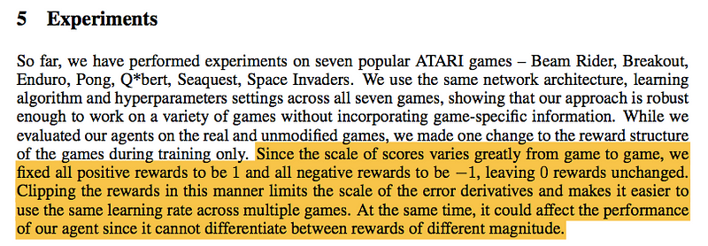
Oooh. First half is self explanatory. The second half tells about one very important thing about this experiment: that the nature of rewards being input to the agent was modified. So, *any* positive reward was input as +1, negative rewards were input as -1, and no change was input as 0. This is of course very different from how real games work — rewards are always changing, and some accomplishments have higher rewards than others. But it’s impressive that in spite of this, the agent performed better than humans in some games!
We’ve already talked about e-greedy (in Section 2), and experience replay. This is about the specific details of their implementation.
More detail about why they use a stack of 4 video frames instead of using a single frame for each state.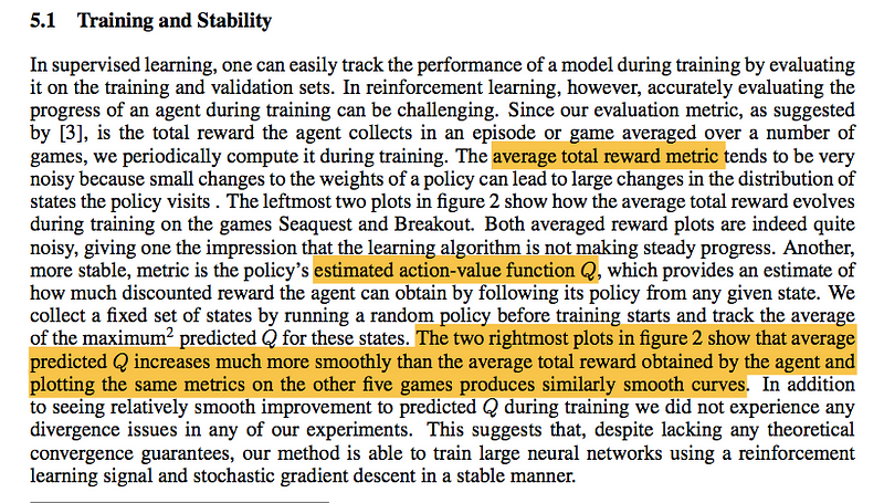
This is about the evaluation metric you use while training. Usually in supervised learning you have something like validation accuracy, but here you don’t have any validation set etc to compare with. So what other things can we use to check whether our network is training towards a point or are the weights just dancing around? Hmmm, let’s think about that. The purpose of this whole paper is to create an AI agent which gets a high score on the game, so why not just use the total score as our evaluation metric? And we can play several games and get the average overall score. Well, turns out that using this metric doesn’t work well in practice, as it happens to be very noisy.
Let’s think about some other metric? Well, another thing we’re doing in this experiment is to find a ‘policy’ which the AI will follow to ensure the highest score (it’s off policy learning, as explained previously). And the Q-value at any particular moment represents the total reward expected by the AI in future. So if the AI finds a great policy, then the Q-value for that policy will be higher, right? Let’s see if we can use the Q-value itself as our evaluation metric. And voila, it seems to be more stable than just the averaged total reward. Now, as you can see there’s no theoretical explanation for this, and it was just an idea which happened to work. (Actually that’s what happens in deep learning all the time. Some things just work, and other things which seem common sense just don’t. Another example of this is Dropout, which is a batshit crazy technique but works amazingly).
This should be self explanatory. It shows how the value function changes in different moves of the game.
Here we compare the paper’s results with prior work in this field. “Sarsa” refers to [s1,a1,r,s2,a2]. It is an on-policy learning algorithm (as opposed to our off-policy) approach. It’s not easy to understand the difference so easily, here’s a good one.
And another.
The rest of this paragraph is quite easy to read.
For this paragraph and everything beyond… ‘Look and marvel at how much better their approach performs!’


